
All you need to know about Normal Distribution

Imagine a bell-shaped curve that appears over and over in different areas like math science and even in everyday life. This curve is called the normal distribution, or sometimes the Gaussian distribution. It’s a special way to understand how numbers tend to group together. This concept is super important because it helps us make sense of data and predict how things behave in various situations. It is a type of continuous probability distribution for a real-valued random variable and is one of the most important distributions in statistics and the natural sciences.
Characteristics of the Normal Distribution
- Symmetry: The normal distribution is symmetric around its mean, with the shape of the distribution identical on either side of the mean.
- Mean, Median and Mode: In a perfectly normal distribution, the mean (average), median (middle value) and mode (most frequent value) are all equal and located at the center of the distribution.
- Bell-shaped curve: The distribution has a distinct bell shape, which is where the alternative name “bell curve” originates. The bell curve is wide in the middle and tapers off at the ends.
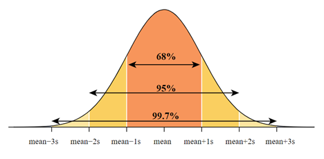
- 68–95–99.7 Rule: This rule, also known as the empirical rule, states that for a normal distribution, about 68% of the data falls within one standard deviation of the mean, 95% of the data falls within two standard deviations and approximately 99.7% falls within three standard deviations.
What are the properties of normal distributions?
The normal distribution is a bell-shaped curve that is symmetric around the mean, which is denoted by the symbol μ. This means that if we draw a vertical line through the center of the curve at the mean, the area to the left of the line is equal to the area to the right of the line.
Since the total area under the curve of a normal distribution is equal to 1, this implies that the probability of a randomly chosen value being above the mean is equal to the probability of it being below the mean.
For example, if the mean of a normal distribution is 50 and the standard deviation is 10, then the probability of getting a value between 40 and 50 is the same as the probability of getting a value between 50 and 60.
This is because the distribution is symmetric around the mean, and the areas under the curve on either side of the mean are equal.
This property of the normal distribution has many important implications in statistics and data analysis. It allows us to make predictions and calculate probabilities based on the distribution of values around the mean, and it forms the basis for many statistical tests and models.
The standard deviation σ determines the spread or variability of the distribution. As the standard deviation increases, the distribution becomes wider. The normal distribution has many useful properties, such as the fact that 68% of the values fall within one standard deviation of the mean, 95% fall within two standard deviations, and 99.7% fall within three standard deviations.
The standard deviation σ is a measure of the spread or variability of the values in a normal distribution. Specifically, it tells us how much the values in the distribution vary from the mean μ.
If the standard deviation is small, then the values in the distribution are tightly clustered around the mean, and the distribution is narrow. Conversely, if the standard deviation is large, then the values in the distribution are more spread out and the distribution is wider.
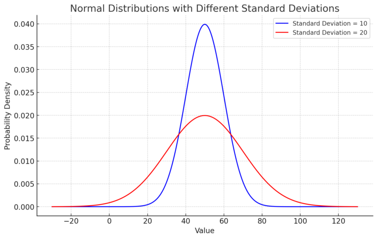
Here’s the graph depicting two normal distributions:
The blue curve represents the distribution with a standard deviation of 10. You can see that its values are mostly concentrated around the mean of 50, primarily between 40 and 60.
The red curve represents the distribution with a standard deviation of 20. This distribution has a broader spread of values around the mean.
As expected, the distribution with a larger standard deviation is wider, indicating greater variability in the data.
The standard deviation is an important parameter in understanding and analyzing data. It can help us identify outliers or unusual values in a dataset, and it is used in many statistical tests and models to quantify the uncertainty or variability in our measurements or estimates.
The total area under the curve of a normal distribution is equal to 1, which means that the probability of any event occurring is always between 0 and 1
Researchers frequently employ a normal distribution to model the behavior of numerous random variables, such as individuals’ heights or weights within a population.
This characteristic goes by the term “normalization condition.” It guarantees that the overall probability of all potential event outcomes equals 1. In simpler words, the curve’s area represents the cumulative probability of all conceivable outcomes, and this probability consistently ranges between 0 and 1.
In statistical analysis, the normal distribution finds frequent use in estimating the probability of a specific event taking place. By calculating the area under the curve between two points on the distribution, we can determine the probability of an event falling within that range. For example, if we want to know the probability of a person’s height falling between 5’6″ and 6’0″, we can use the normal distribution to calculate this probability.
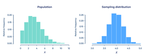
Central limit theorem
It states that the sum or average of a large number of independent and identically distributed random variables tends to follow a normal distribution.
The central limit theorem is a fundamental concept in probability theory and statistics. It states that, under certain conditions, the sum or average of a large number of independent and identically distributed (i.i.d.) random variables tends to follow a normal distribution, even if the individual variables themselves are not normally distributed.
The conditions required for the central limit theorem to hold are:
- The random variables must be independent and identically distributed (i.i.d.).
- The sample size must be sufficiently large (usually, n ≥ 30).
- The random variables must have finite mean and variance.
When these conditions are met, the distribution of the sample mean or sum will be approximately normal, regardless of the underlying distribution of the individual variables. This is particularly useful in practical applications, where the individual variables may have complex and unknown distributions, but the properties of the sample mean or sum can be easily calculated using the normal distribution.
The central limit theorem has important applications in many fields, including finance, physics, engineering and social sciences. It provides a theoretical justification for using statistical inference techniques, such as hypothesis testing and confidence intervals, based on the assumption of normality.
Testing for Normality
Testing for normality is crucial before making assumptions and applying statistical tests. Various techniques can be used to check this, such as QQ-plots, the Shapiro-Wilk test and the Kolmogorov-Smirnov test.
A QQ-plot, or quantile-quantile plot, compares two probability distributions by plotting their quantiles against each other. If the data follows a normal distribution, the points in the QQ-plot will approximately lie on the line y = x.
The Shapiro-Wilk test and the Kolmogorov-Smirnov test are statistical methods used to examine whether a dataset adheres to a specific expected pattern. In both tests, the null hypothesis assumes that the data originates from a population with a known distribution. When the computed p-value falls below the predetermined significance level (usually 0.05), this leads to the rejection of the null hypothesis, indicating that the data does not exhibit characteristics of a normal distribution.
When Data Is Not Normally Distributed
There are many scenarios where data may not follow a normal distribution. For instance, economies often exhibit right-skewed income distributions, where many individuals earn a small amount of money, and only a few earn a substantial sum. In such scenarios, practitioners turn to alternatives to standard methods. They employ non-parametric statistical tests that avoid assuming a specific data distribution. Examples include the Wilcoxon signed-rank test for matched pairs of observations and the Mann-Whitney U test for independent observations.
Applications of the Normal Distribution
It is commonly utilized in both natural and social sciences as a means to represent random variables with real values when the exact nature of their distributions is unknown. It serves as a good approximation for a variety of phenomena, including:
- Test Scores: Educational systems often assume that student performance follows a pattern similar to the bell-shaped curve. This simplifies grouping students into categories like “above average,” “average,” or “below average.”
- Measurements: Physical attributes such as height, weight, or blood pressure within a group of individuals tend to exhibit a similar bell-shaped pattern.
- Quality Control: Numerous manufacturing and business processes adopt this curve to assess variations and ensure quality standards.
- Stock Market Returns: In the realm of finance, the returns on stocks or portfolios frequently exhibit a propensity towards a bell-shaped curve pattern.
The normal distribution is not just a cornerstone of statistics; it is a fundamental tool that permeates many scientific disciplines and everyday applications. Its universal nature allows us to make sense of patterns and behaviors in diverse fields, from education and healthcare to manufacturing and finance.
Understanding its characteristics, uses, and importance can greatly enhance our understanding of the world. As we continue to gather and analyze data, the normal distribution will undoubtedly remain a valuable tool, guiding us to the path of new discoveries and insights.